Steelmaking scheduling optimization - MIP implementation (Part 1)
Introduction
A tricky aspect within the field of operations research is reproducing the work of other researchers. One of the biggest obstacles is that source code is rarely provided (I am part of this problem – though for confidentiality reasons beyond my control). While it serves as an excellent learning opportunity, reproduction demands significant effort.
To explore this, I will consider a recent paper from the steelmaking-continuous-casting (SCC) literature:
- Juntaek Hong, Kyungduk Moon, Kangbok Lee, Kwansoo Lee & Michael L. Pinedo (2022) An iterated greedy matheuristic for scheduling in steelmaking-continuous casting process, International Journal of Production Research, 60:2, 623-643, DOI: 10.1080/00207543.2021.1975839
My goal is not to reproduce their results exactly or verify their claims, but rather to illustrate the effort and pitfalls of reproducing literature models. In the future, I want to integrate this model with ladle dispatching decisions to answer a few lingering questions from my own research. Moreover, I am restricting myself to open-source solvers to evaluate how competitive they are when tackling the SCC problem.
In this first part of the series, I will share some practical tips and the results of implementing a MIP model described in an academic paper. The full source code is available in this github repository.
Problem description
First things first, I will provide a brief introduction to the problem at hand. A more complete description can be found in the paper used throughout this post.
Steel is produced in two main routes: the integrated and electric routes. In the integrated route, hot metal is charged into a BOF (Basyc Oxygen Furnace) along with a small percentage of scrap to produce crude steel heat. Alternatively, scrap can also be molten into an EAF (Electric Arc Furnace) with the same end goal – this is the electric route.
The crude steel is then tapped into a steel ladle and proceeds to the secondary refining stages. It can include a stirring station, ladle furnace and vaccum degasser, for example. A steel grade defines the temperature and quality specifications, which in turn defines which routes (sequence of stages) a heat must undergo until casting. Finally, the continuous casting process is reached, where the molten steel is loaded into a tundish and then solidified into a water-cooled mold to produce slabs.
A particularity of the SCC scheduling problem is that heats in a cast must be processed continuously – which makes it more complicated than typical flow-shop scheduling formulation. Several formulations of this problem have been proposed in the literature. Heuristics are mostly employed to obtain high-quality solutions for practical instances.
Implementation
Academic papers typically begin by establishing a mathematical description of the problem: sets, parameters, decision variables, constraints, and objectives. Implementation is usually straightforward from this description using any modeling language. I personally prefer pyomo because it does not bind me to a specific solver interface. Of course, it does add an overhead each time an instance is built, and it lacks some advanced features available in a solver’s native interface.
In the following subsections, I share a few insights gathered during the implementation.
Input data structure
Before implementing the mathematical model, I like to create a consistent data model that is easy to serialize in a text file (JSON, YAML, etc.) and represents the problem’s structure. pydantic is very interesting for this step, especially because python does not strongly enforce types.
Below is an example used for implementing the SCC problem. Notice that there is a clear connection to the actual notation and parameters used in the manuscript. Moreover, the data transformation logic is neatly contained within the data classes. This segregates data preprocessing from modeling logic, making each part easier to test and maintain individually while preventing the mixing of data processing with mathematical expressions.
from pydantic import BaseModel

class SCCData(BaseModel):
    casts: dict[int, Cast] = {}
    stages: dict[int, Stage] = {}
    penalty_tardiness: float
    penalty_earliness: float
    penalty_idle_time: float
    penalty_cast_break: float
    max_wait_time: int

    @property
    def charge_indexes(self) -> list[int]:
        """Return a list of all charge IDs."""
        return [charge.id for cast in self.casts.values() for charge in cast.charges]

    def charge_stages(self, charge_id: int) -> list[int]:
        """Return a list of stage IDs for the given charge ID."""
        for cast in self.casts.values():
            for charge in cast.charges:
                if charge.id == charge_id:
                    return [stage.id for stage in charge.steel_grade.route]
        raise ValueError(f"Charge ID {charge_id} not found in any cast.")
Working with pyomo Sets
A pyomo feature that I particularly enjoy is using sets to construct the model. For me, the hardest part of implementation is getting comfortable with the paper’s mathematical notation, and utilizing set notation is quite handy for translating a mathematical expression into Python code. Take Equation 4 from the paper as an example:
To avoid getting lost in the notation and repeating code, I isolate the sets from the mathematical expressions to keep things clean. This also allows me to reuse the exact same set to build similar constraints (such as Equation 3 in this example):
# set definition for Equations (3) and (4)
model.CHARGE_CHARGE_STAGE_INTERSECTION = pyo.Set(
            initialize=[
                (charge1, charge2, stage_id, machine_id)
                for charge1 in data.charge_indexes
                for charge2 in data.charge_indexes
                for stage_id in data.stages.keys()
                for machine_id in data.machine_indexes
                if stage_id in data.charge_stages(charge1)
                and stage_id in data.charge_stages(charge2)
                and machine_id in data.machine_indexes_per_stage[stage_id]
                and charge1 != charge2
            ]
        )

# add constraints (3) to the model
model.constraint3 = pyo.Constraint(
            model.CHARGE_CHARGE_STAGE_INTERSECTION,
            rule=lambda m, k1, k2, s, i: (
                (m.x[k1, k2, s] + m.x[k2, k1, s] >= m.y[i, k1, s] + m.y[i, k2, s] - 1)
                if k1 < k2
                else pyo.Constraint.Skip
            ),
        )

# add constraints (4) to the model
model.constraint4 = pyo.Constraint(
            model.CHARGE_CHARGE_STAGE_INTERSECTION,
            rule=lambda m, k1, k2, s, i: (
                m.x[k1, k2, s] + m.x[k2, k1, s] <= 1 - (m.y[i, k1, s] - m.y[i, k2, s])
            ),
        )
While other efficient approaches certainly exist, a key takeaway here is that a modeling framework supporting native set operations should be heavily leveraged. Pyomo handles this beautifully once you grasp its syntax.
Validation
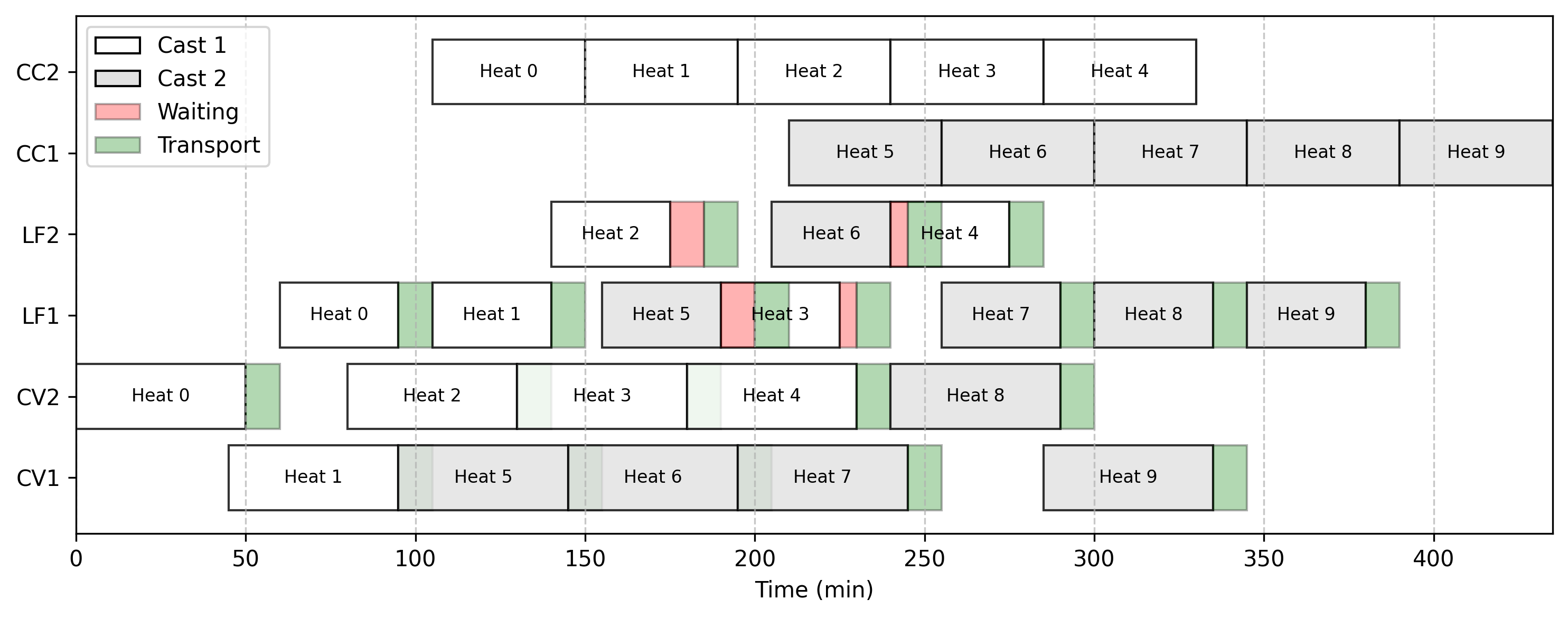
I usually can implement an initial version of the model very fast – specially with AI coding assitants. However, it is often wrong or infeasible. Hence, I start with a small valid instance based on information present on the manuscript for validation. For scheduling problems, I find Gantt charts especially useful for validation model outputs. An example is displayed below, considering a small scenario with 2 casts, 10 heats, 3 stages and 2 machines per stage. It is possible to see that the stages are in order, casts are continuous, and that waiting and transportation times are also consistent. From the results, it is possible to confirm that the implementation is correct.
I also xperimented with unit testing the model implementation, which is something that had been on my wind for some time. However, it became evident quite early that comprehensive testing (especially for asserting mathematical expressions) would require much more effort than what I wanted. Therefore, I kept it simple: I only ensured that the correct number of variables and constraints were added to the model. This doesn’t guarantee that the outputs are correct, but allows to quickly catch basic modeling mistakes. Ideally, the next step was to ensure that all the equations were correct (objectives and constraints) after initializing the model with a valid solution. I think unit testing optimization mdoels is a very interesting topic on its own, maybe I will dig more into this later.
Results
While my primary goal isn’t to benchmark model performance, I did want to see how well open-source solvers scale with instance size. Using the same plant configuration described above, I generated small and medium synthetic instances based on the parameters provided by the authors (they are available for download here as LP files). The termination criteria were set to a 0.01% optimality gap or a 15-minute runtime limit. The primary metrics are summarized in the table below.
While my primary goal isn’t to benchmark model performance, I did want to see how well open-source solvers scale with instance size. Using the same plant configuration described above, I generated small and medium synthetic instances based on the parameters provided by the authors (they can be downloaded here as LP files). The termination criteria were set to a 0.01% optimality gap or a 15-minute runtime limit. The primary metrics are summarized in the table below.
| Problem Instance | HiGHS | SCIP | |||
|---|---|---|---|---|---|
| Casts | Heats | Time (s) | Obj Value | Time (s) | Obj Value |
| 1 | 3 | 0.05 | 225.0 | 0.13 | 225.0 |
| 1 | 4 | 0.13 | 240.0 | 0.20 | 240.0 |
| 1 | 5 | 0.37 | 255.0 | 0.65 | 255.0 |
| 1 | 6 | 1.70 | 270.0 | 1.22 | 270.0 |
| 2 | 3 | 18.6 | 64.99 | 2.4 | 64.99 |
| 2 | 4 | 900.1 | 69.99 | 519.3 | 65.39 |
| 2 | 5 | 900.1 | 79.99 | 900.3 | 65.43 |
| 2 | 6 | 900.1 | 90.0 | 900.3 | 83.04 |
| 3 | 3 | 900.0 | 59.99 | 209.5 | 60.0 |
| 3 | 4 | 900.2 | 44.99 | 900.7 | 57.49 |
| 3 | 5 | 900.4 | 64.99 | 900.2 | 52.5 |
| 3 | 6 | 900.3 | 72.49 | 901.0 | 82.47 |
What stands out immediately is how quickly the model becomes intractable (which isn’t a surprise). We can also see that while both solvers yield similar outcomes, one may reach a slightly better solution than the other depending on the specific instance. Of course, this isolated experiment isn’t enough to claim overall superiority for either solver – but that was not the objective anyways.
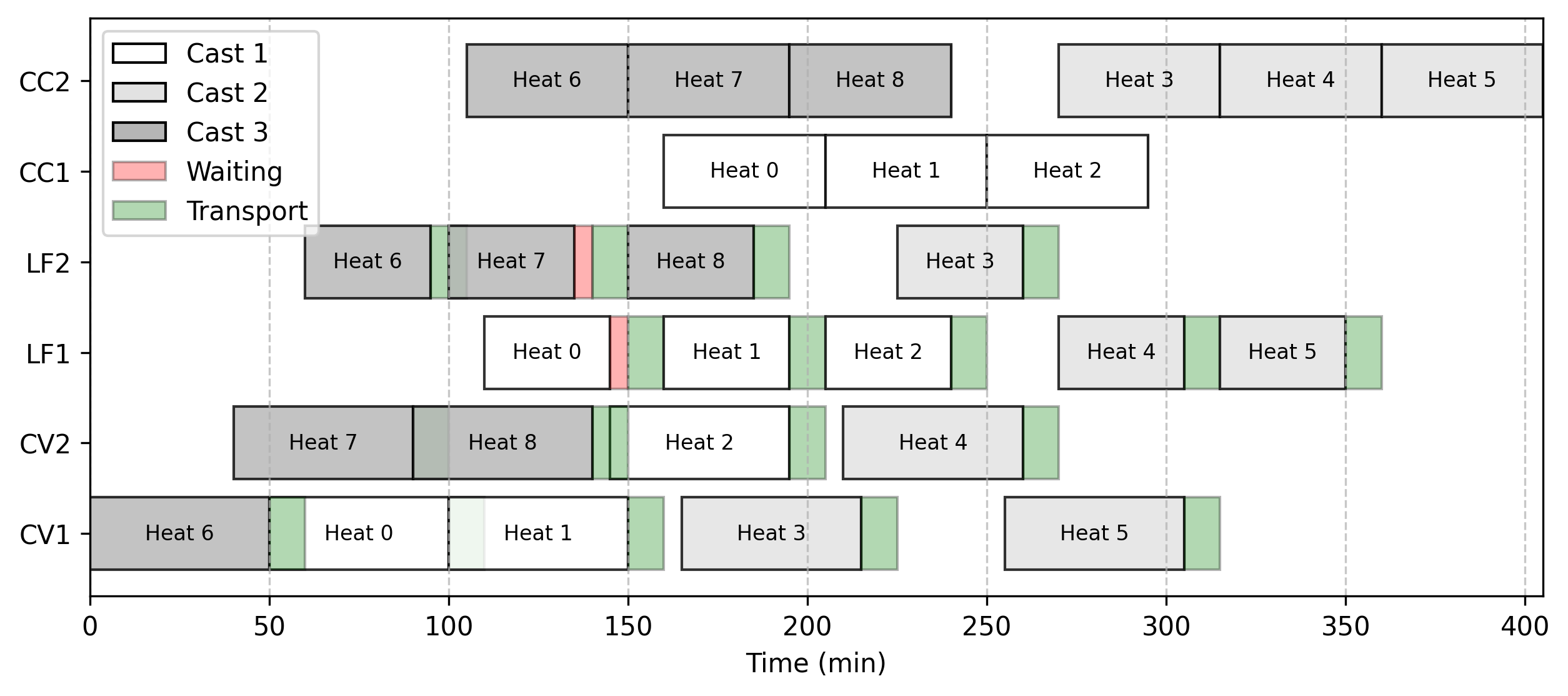
However, one characteristic of this model is its high degree of symmetry. Take the instance with 3 casts and 3 charges: both solvers discover the exact same objective value, but HiGHS is unable to prove optimality within the 15-minute time limit. Examining the Gantt charts for these solutions reveals the extent of this behavior: delays match closely, but the casts finish in a completely different order, yielding an identical overall completion time (makespan).
| SCIP | HiGHS |
|

|
|---|
I haven’t found much literature exploiting this specific symmetry to optimize exact SCC solution performance (perhaps I just haven’t looked hard enough), though it has been studied extensively for generic scheduling formulations. Most authors bypass exact methods entirely and jump straight to heuristics when tackling this problem. Yet, there may still be a valuable opportunity to strengthen existing formulations and leverage recent performance leaps in MILP solvers.
Ultimately, optimality might not even be vital for practical operations. Real-world parameters are naturally uncertain, and solutions close to the theoretical optimum often function identically in practice.
Conclusions
The model works exactly as described in the paper. However, there are a few practical gaps that require careful troubleshooting, such as calculating tight Big-M coefficients. While you can deduce these parameters once you understand the mathematical expressions, explicitly stating them in the manuscript would save a lot of time.
Moreover, the high degree of symmetry present in the continuous casting problem means that exact solvers quickly hit a wall, spending valuable time trying to prove theoretical optimality for schedules that look almost identical in practice.
Because seeking exact optimality becomes intractable so quickly, practical applications almost always rely on alternative solution strategies. In the next post, I will share the implementation of the iterated greedy matheuristic proposed by the authors. We will see how combining heuristic search with localized mathematical programming allows us to break through these tractability limits—and bring us one step closer to integrating ladle dispatching decisions!
This work is licensed under CC BY-NC 4.0